Static or Dynamic? It is a matter of balance

Now that we know how to identify parallel parts of our program, the question is now what to do with this knowledge. Or, how do you write a parallel program. To answer this question, we will discuss what the structure of a parallel program may look like. Programs can be organized in different ways. We already discussed SPMD (Single Program Multiple Data) and MPMD (Multiple Programs Multiple Data) models. SPMD and MPMD represents the way a program looks from the point of view of the cluster. Note, that using a MPMD model with MPI an "app" or "procgroup" file will be needed to start different programs on cluster nodes. Let's see what the programs look from the implementation standpoint.

There are a variety ways to structure parallel codes. In this article we explore three common models that have been successfully used in tools like BERT 77, a Fortran conversion tool. As we know,a parallel program may contain different concurrent parts. When making these parts parallel one may find that the processor load may vary quite a bit. We will ignore data transfers, and only look at the efficiency of the parallel code, i.e. load balance.

An Example

 CALL S1(X)
 DO I = 1, N
    CALL S2(Y(I))
 ENDDO
 CALL S3(Z)

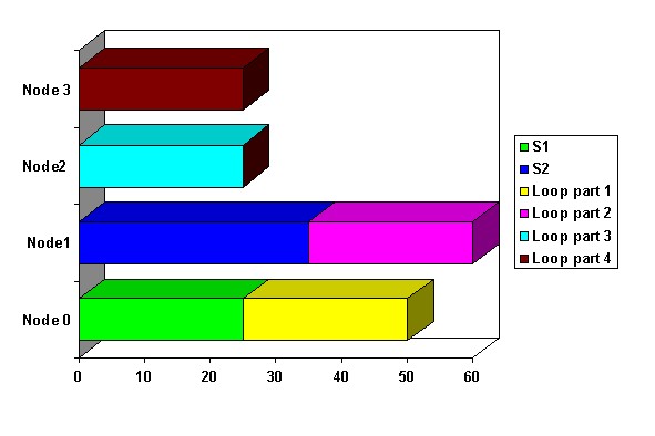
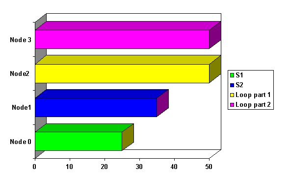
These subroutines have no side effects, and our program has three independent parts: CALL S1, CALL S3 and the DO LOOP. We also assume the loop is concurrent. The execution times are as follows:

If we add up the component times we see that the sequential execution time is 160 ms. The question is: How to use four nodes to get smaller execution time? When we make straight forward parallelizations, we get the workload represented in figure one.

Figure One: Processor Load for Naive Parallelization

Now we get an unimpressive runtime of 100 ms instead of 160 ms. Let's see if we can do better.

Balancing with Data Flow

The master dynamically splits parallel parts of the program based on the number of workers. When a worker starts, all data required for its execution are sent from the master to the worker. When the worker is finished, all results are sent back to the master. In our case, the program can be decomposed as shown in Figure Two.

Figure Two: Program Decomposition for a Flow model

In the figure, m is number of parts into which the DO loop is decomposed. An example of the time diagram with four nodes and loop split in four parts (m = 4) is given in Figure Three. In the figure, three nodes start to execute worker1, worker 2, and worker3.1. The first, Node 1 finishes worker1 and starts worker 3.2. Then Node 3 finishes worker 3.1 and starts worker 3.3. Finally, Node 2 finishes worker 2 and starts worker 3.4.

Figure Three: Balancing between nodes

As you can see, the execution time is reduced to 60 ms. This is much better! The foloowing sidebar shows a template for a flow type programs.

  n_workers = m+2
  balance workers to workload
  do k = 1, n_nodes
    transfer data to node k
  enddo
  do k = n_nodes+1, n_workers
    wait for a worker to finish
    receive data from worker w
    transfer data to worker w
  enddo
  do k = 1, n_nodes
    wait for finishing worker
    receive data from worker
  enddo

  do while(not_finished)
  receive job from master
  if(job .eq. job1) then
     receive x
     call s1(x)
     send x to master
  elseif (job .eq. job2) then
   receive imin, imax, y(imin: imax)
   do i =imin, imax
   call s2(y(i))
   enddo
   send y(imin: imax)
  elseif (job .eq. job3) then
    receive z
    call s3(z)
   send z to master
  endif

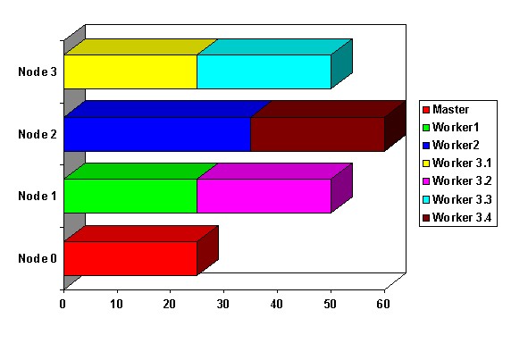
As you can see in the program, master assigns jobs to first n_nodes workers. Then the master monitors the state of the workers. When a worker finishes, the master assigns another job to a worker. When all the jobs are assigned, the master simply waits for the remaining data.

Be Dynamic

  IF(master) THEN
      n_parts = n_workers = m+2 ! compute number of
                                ! parallel parts
      DO i_part=1, n_workets
         receive data from worker w
         load_worker(w)     ! send to worker next 
                            ! portion or end signal
      ENDDO
   ELSE
      work = .true.
      DOWHILE(work)
         compute (first time) or receive next part
         goto (1, 2, 3, 4), part
1        receive x from master
         call s1(x)   ! first part (block)
         send x to master
         goto 5
2        receive imin, imax, y(imin:imax) from master
         DO i = imin, imax
     call s2(y(i))
     ENDDO
     send y(imin:imax) to master
         goto 5
3        receive z from master
         call s3(z)   ! first part (block)
         send z to master
         goto 5
4        work = .false. ! end of work
5        CONTINUE
      ENDDO
   ENDIF
   broadcast(x, y, z)   ! broadcast from master to all

The load balance of the dynamic algorithm is practically the same as with the flow model. Which model is best to use? The answer depends on how much data is used and how much data is produced by the parallel segments.

The Static Model

The static model is based on array distribution and is probably the most common model used for parallelization. This strategy means that arrays are split between computational nodes, and operations are performed on these elements on specific nodes. For example the following code fragment can be executed with a static model.

REAL Y(N)
  ... 
DO I = 1, N
  CALL S2(Y(I))
ENDDO

A static parallelization is shown in the sidebar.

! suppose that n is divisible by n_nodes
real y(n/n_nodes) 
  ... 
low = P*(n/N_nodes)+1
if(current_node .eq. node1) then
  s1(x)
else if(current_node .eq. node2) then 
  s3(z)
endif
high = (P+1)*(n/N_nodes)
do I = low, high
  call s2(y(I- P*(n/N_nodes))
enddo

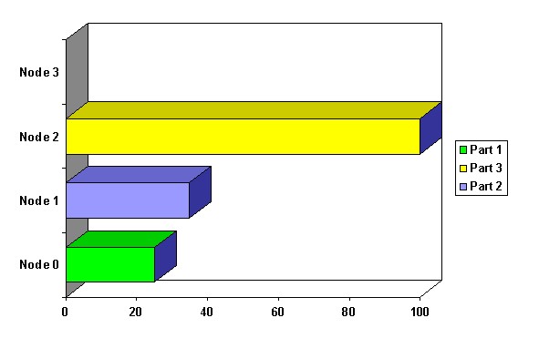
In general, as the number of nodes increases, the amount of memory needed per node decreases because smaller portions of the array are placed on each node. Let's look again at the program. With a static parallelization we can assign S1 to Node 1 and S3 to Node 3 as before. We will then distribute array Y on all four nodes. Figure Four shows this distribution.

Figure Four: Static array distribution on four nodes

We get 60 ms again. Can we do better? Another way is to distribute the array is on a subset of nodes, in this case two nodes. Then for the same program we can get the following diagram.

Figure Five: Static array distribution on two nodes

Now we got 50 ms for the program. This result is a good, but the price one has paid for this model is that the balancing of parallel loops is more "rigid" than you may like.

A Recap

The Dynamic model programs are executed as SPMD and like the Flow model there is no partitioning. Each node, including the master, has the same program. All nodes are kept up to date at the completion of each parallel part of the program. The scheduling is dynamic and the size of the problem is limited by the size of a node because the entire program and data must fit on each node.

The Static model is SPMD as well, however, the data is partitioned across nodes. The scheduling is static and thus could have lower efficiencies if loop boundaries change from run to run. (i.e. The program is committed to parallel execution at certain points in the program) The size of the program can be very large as the data are sliced and placed on different nodes.

This article was originally published in ClusterWorld Magazine. It has been updated and formatted for the web. If you want to read more about HPC clusters and Linux, you may wish to visit Linux Magazine.

Pavel Telegin is currently Department Head of Programming Technology and Methods in the Joint Supercomputer Center, Moscow, Russia.