Adding water and proteins to your cluster (virtually)

GROMACS is a powerful and versatile package designed to help scientists simulate the behavior of large molecules (like proteins, lipids, and even polymers). Naturally, calculations of such magnitude require the computing horsepower provided by HPC clusters.

Superficially, molecular simulation is really a strikingly simple idea. Given a collection of atoms like a box of water or a protein, we would like to calculate how they interact and move under realistic laboratory conditions. The catch is that it can require truly insane amounts of computational power. Fortunately, relatively few processes (apart from bond breaking/formation) require any quantum mechanical treatment, so we can model atoms as simple classical particles and apply Newton's equations of motion. The expensive part is to determine the force on each atom, since it depends on the positions of all other atoms in the system -- even for a small water box this can involve millions of floating-point operations. Once the forces are known it is straightforward to calculate how the atoms move and where they will be at the next step. Sounds fairly easy, right?

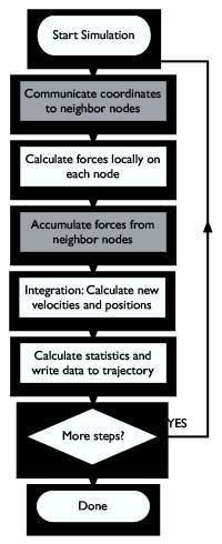
Ah, but the problem is that a step only simulates femtoseconds of real time, so we need to perform five million steps like this to reach 10 nanoseconds -- and that's still the very low end of chemically interesting timescales! This is where the clusters enter -- by parallelizing the algorithm to use multiple processors we can reduce the runtime from months to weeks or even days. Figure One shows a rough sketch of how the parallelization works. This article will step you through installation and basic use of the Gromacs molecular simulation and analysis package, and provide some tips on how you can improve parallel performance. Enough smalltalk, let's get started instead!

Installation & Setup

We'€™ll assume that you have an account on a cluster, and that your home directory is mounted on all nodes. You will also need an MPI library to do parallel communication; the command which mpicc should echo the location of the MPI-enabled compiler if it is in your path. If you can't find it, read the performance tuning section at the end of this article for instructions on how to compile your own optimized MPI library -- you will probably end up doing that pretty soon anyway. Most users don't have root access, so instead of using the RPM packages from the Gromacs Site, we'll show how to compile the software yourself and install it in your home directory.

Compiling FFTW

Some options in Gromacs (notably PME electrostatics) only work if we install the free FFTW library to provide Fourier transforms. Some Linux distributions ship FFTW by default, but you might need to recompile if you change the MPI library as described elsewhere in this article. Download the source code fftw-2.1.5.tar.gz from the FFTW site or our website. Note that FFTW version 3.x won't work since it doesn't support MPI parallel transforms yet. Unpack the tarball with

tar xzf fftw-2.1.5.tar.gz

Change to the new directory and configure it as

./configure --prefix=/home/joe/software  \
      --enable-float               \
            --enable-type-prefix         \
            --enable-mpi

The backslashes just mean everything should be on a single line. Replace /home/joe with the location of your own home directory, or skip the prefix option if you have root access and want to install FFTW under /usr/local. When the configuration is ready, issue make and make install to compile and install everything.

Compiling Gromacs

Just like FFTW, Gromacs uses standard GNU autoconf scripts, so the installation is straightforward, even when compiling for a parallel architecture. Download the latest source code from the Gromacs website, and unpack it just like we did for FFTW above. If you installed FFTW in your own directory we need to set some environment variables to tell the configure script where to find the headers and libraries. If your shell is bash or csh (echo $SHELL to find out) this is done as

export CPPFLAGS=-I/home/joe/software/include
export LDFLAGS=-L/home/joe/software/lib

or, if you use the csh/tcsh shells:

setenv CPPFLAGS -I/home/joe/software/include
setenv LDFLAGS -L/home/joe/software/lib

If you already had FFTW installed in /usr or /usr/local you don't need to do anything. Continue and configure Gromacs as

./configure --prefix=/home/joe/software \
            --enable-mpi \
            --without-x

Many clusters only have X libraries installed on the frontend, so if we don't disable X support the binaries might not work on the compute nodes. You can also try to add the option €“--enable-all-static to link all libraries (e.g. FFTW) statically, but this will only work if static system libraries are available. Build and finish the installation with the standard make followed by make install. By default the Gromacs binaries and libraries will be placed in a subdirectory named after the current architecture, so if you have a mixed cluster you can install all different versions in the same place. You might want to add this binary directory to your path.

Other Programs

In this tutorial we will use two very nice visualization programs that interface well with Gromacs. We use them a lot in our daily simulation work, so it is a good idea to install them locally on your workstation (not the cluster, since we need OpenGL support):

• Grace, a 2D graphing program for the X Window System and Motif.
• Pymol, a powerful OpenGL-based molecular viewer by Warren DeLano.

Puh! That was the boring part, now we can start to play with our new software toys!

Starting Parallel Jobs

The exact way to get a parallel environment depends on whether your cluster has any batch queue system, and which MPI library is installed. The most common free batch system is PBS or Torque (descendant of PBS), where you can request e.g. 4 interactive-use nodes for two hours with the command

qsub -l nodes=4,walltime=2:00:00 -I

The normal usage is to provide a script file with commands to execute instead of the -€“I option, but for testing it is nice not having to wait in the queue again each time you make a small mistake. The first thing to do on the nodes is to start the MPI environment. For LAM/MPI it is done as

lamboot -v $PBS_NODEFILE 

PBS_NODEFILE is an environment variable provided by PBS and Torque, it is the full path to a file that contains the hostnames of the processors allocated to your job. If you just have a very small cluster without any queue system you replace this with your own hostfile where you list the hostname of the nodes to use once for each CPU on them.

A Simulation Project

Our first task is to find something to simulate. Gromacs includes coordinates for water and some other simple molecules, but we will download a hen eggwhite Lysozyme structure to have something slightly more interesting, it is a well-known protein with 164 residues. Before we execute any Gromacs programs we'll do something neat. Issue the command:

source /path/to/gromacs/bin/directory/GMXRC

You now have shell completion both for Gromacs executables, options, and data files, as well as manual pages (try “man pdb2gmx”). It works for all normal Unix shells, so you probably want to add it to your login file. You can get also instant help with the -h option to any Gromacs command.

Preparing a Protein Structure

Go to the Protein Data Bank, and enter 2LZM in the search box. Tick the field for “PDB ID” and hit the button. Select download, and get the uncompressed PDB file (upper left entry in the second table). Create a new directory under your home directory on the cluster and copy the file 2LZM.pdb to it. This PDB file is just a collection of atomic coordinates and names, but it doesn'€™t contain any definitions of which parameters to use in a simulation. We will use the Gromacs program pdb2gmx to select a set of parameters (force field), and automatically translate the PDB file to (1) a topology file that describes all static properties like connectivity, bond parameters, names, etc., and (2) a coordinate file. This program doesn't need any parallel environment, so just execute

pdb2gmx -f 2LZM.pdb

Select the OPLS-AA/L force field when asked, and press return. You can set the output file names with other flags, but for now we'll stick to the default names. The topology will be called topol.top, coordinates conf.gro, and the file posre.itp contains something called position restraint data (we will use it later). A protein in vacuum isn't particularly realistic though, so we want to use periodic boundary conditions and add solvent water around it. Gromacs supports all types of triclinic boxes, but let's keep it simple. We center the protein in a rectangular box with at least 0.5 nm from the atoms to the box edge, and write it to a new file:

editconf -f conf.gro -€“d 0.5 -o newbox.gro

Now we can add water to our modified coordinates with the program genbox. We use the SPC water model here -- the coordinates spc216.gro will be read from the Gromacs library directory, and if you provide the topology file it will automatically be edited to add the new water. We will also show another trick: all Gromacs programs detect a number of file formats automatically, so it is just as easy to write the coordinates in PDB format instead of .gro (PDB files cannot store velocities, but we don't have any yet):

genbox -cp newbox.gro -cs spc216.gro -€“p topol.top -o solvated.pdb

Genbox will output a lot of information and echo that it added about 4400 water molecules in your box. Are you itching to see what the coordinates look like? Copy solvated.pdb to your workstation and display it with pymol solvated.pdb.

Energy Minimization

Before we start any simulations we need to remove possible clashes between atoms by energy minimization,€“ otherwise the structure would just explode if there are overlapping atoms. Create this parameter file called em.mdp in your favorite editor:

integrator  = cg
nsteps      = 250
nstxout     = 0
nstvout     = 0
nstlog      = 0 
nstenergy   = 0
rlist       = 1.0
coulombtype = cut-off
rcoulomb    = 1.0
vdwtype     = cut-off
rvdw        = 1.0
constraints = none
define      = -DFLEXIBLE

In short, this means we will use a conjugate-gradients minimizer, use standard interactions with cut-offs at 1.0 nm, but don't output any data since we just want the final structure. Since we just want to get rid of bad contacts and aren't interested in any true energy minimum we just run 250 steps,“ it is not even worth doing in parallel, although it would work. Prepare a run input file with the command

grompp -f em.mdp -p topol.top -€“c solvated.pdb -o em.tpr

If you had forgotten e.g. what you called your coordinate file you could just hit the tab key after an option to get a list of the files in the current directory that are compatible with it, provided you sourced GMXRC as we recommended! The file em.tpr contains everything we need for the simulation, so you could also prepare everything on your own workstation and just copy run input files to the cluster or supercomputer (portable across different endian architectures and precisions). It will warn you about the system having non-zero charge since we did not add any counter ions, but we'll live with that for the tutorial. We perform the minimization with the mdrun command:

mdrun -v -deffnm em

The -v flag enables verbose output, and the -deffnm flag is a nice shortcut to use em.* for all filename options. The run input file will be read from em.tpr, final coordinates written to em.gro, the energy file to em.edr, etc. The minimization will take about a minute on a modern CPU, and finish with a warning that it did not converge in 250 steps -- that's quite OK.

Position Restrained Dynamics

Next we will start a real simulation, but we will be a bit careful and restrain the protein atoms while we give our new water molecules a chance to relax around the protein. Create a new parameter file pr.mdp:

integrator  = md
nsteps      = 5000
dt          = 0.002
nstxout     = 0
nstvout     = 0
nstlog      = 0
nstenergy   = 0
rlist       = 1.0
coulombtype = cut-off
rcoulomb    = 1.0
vdwtype     = cut-off
rvdw        = 1.0
tcoupl      = berendsen
tc-grps     = system
tau-t       = 0.1
ref-t       = 298
gen-vel     = yes
gen-temp    = 298
constraints = h-bonds
define      = -DPOSRES

We are now using the molecular dynamics integrator, and taking 5000 steps of length 2 fs each. This step length requires bonds involving hydrogens to be kept constant. Atom velocities are generated from a Maxwell distribution at 298K, and during the simulation the temperature will be coupled to 298K using the Berendsen algorithm. Finally we enable position restraints. This time we will prepare a parallel run input file for 4 CPUs:

grompp -f pr.mdp-p topol.top -c em.gro -o pr.tpr -“np 4

Time to put that cluster to use! Request four processors for interactive use, and start MPI on them as we described above, or use the instructions for your own cluster. Since we need to start mdrun on all machines you must provide the full path to the command unless it is in your path, sourcing GMXRC only affects the node you are currently logged in to. Almost all MPI implementations use mpirun to start parallel jobs, so the command to use is normally:

mpirun -np 4 /path/to/mdrun -v -deffnm pr

We still have verbose output, so you will get a message every 10 steps telling you when the simulation is expected to finish -- it should only take a couple of minutes.

The Production Simulation

After the position restrained equilibration has finished it is time for the real simulation where we will collect data to analyze. We will disable position restraints, generate more output data, and use the velocities from the end of the last simulation (saved in the .gro file) instead of generating new ones. The contents of run.mdp is:

integrator  = md
nsteps      = 50000
dt          = 0.002
nstxout     = 10000
nstvout     = 10000
nstxtcout   = 100
nstlog      = 1000
nstenergy   = 100
energygrps  = protein sol
rlist       = 1.0
coulombtype = cut-off
rcoulomb    = 1.0
vdwtype     = cut-off
rvdw        = 1.0
tcoupl      = berendsen
tc-grps     = system
tau-t       = 0.1
ref-t       = 298
constraints = h-bonds

The total simulation time is 100 ps (50,000 steps), which is still very short but enough for a tutorial. Every 10,000 steps we save full precision coordinates and velocities to the trajectory run.trr so we can restart the simulation if something goes wrong, and every 100 steps we will write compressed coordinates to run.xtc (10 times smaller than general trajectories). Energies and similar data like pressure is written every 100 steps to run.edr, and energy terms are written separately for all combinations between protein and solvent groups. Generate the run input file:

grompp -f run.mdp -p topol.top -c pr.gro -o run.tpr -np 4

This simulation will take a while, so let's create a script so it can be submitted as a batch job. The PBS/Torque options can be embedded as a comment in the script, and since most clusters have SMP nodes we ask for 2 nodes and 2 processors per node:

#PBS -l nodes=2:ppn=2
lamboot -v $PBS_NODEFILE
cd /your/project/directory
mpirun -np 4 /path/to/mdrun -deffnm run
wipe

Make the scriptfile executable, and submit the job as qsub scriptfile. Go and have a cup of coffee while you swear over other users competing for resources, and when you are back the output files should be ready in your project directory. All Gromacs binary files are portable, so if you want to you can copy the results and do all post-run analysis on your workstation if Gromacs is installed there.

Analyzing The Energy File

The Gromacs energy files are a bit special in that they store partial sums of energy terms. If you used nstenergy=100 the instantaneous values are written every 100 steps, but the averages and drift statistics we extract from the file are still exact and based on every single step in the simulation. This even works if you are analyzing parts of a simulation, for instance the interval 5.0-10.0 ps in our production run. Use the Gromacs program g_energy to extract data from energy files:

g_energy -f run.edr

You will be presented with a table of different energy terms, pressures, temperature, etc. Select a couple of terms you are interested in and finish with 0. g_energy will write the average, fluctuation and systematic drift to the screen, and generate the plotfile energy.xvg. Remember that we talked about the Grace program before? If you installed it you can simply type

xmgrace -nxy energy.xvg

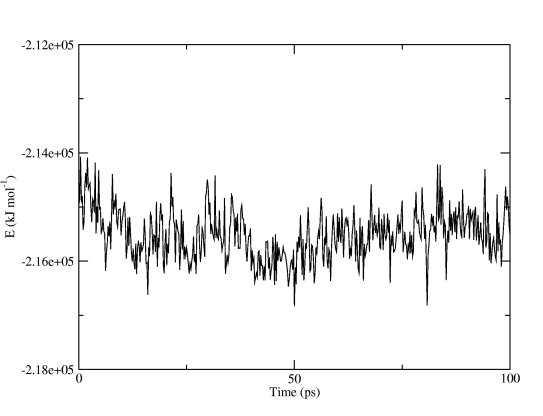
and you will get a finished graph with captions and legends. Figure Two shows the total potential energy, all we did in Grace was to make the graph a little wider. You can even use the command line options to xmgrace and produce postscript or PDF plots automatically!

Analyzing Trajectories

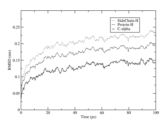
What else can we do? Well, a common property to be interested in is the RMSD variation of atoms with respect to the initial structure. Let's generate it from the trajectory:

g_rms -s em.tpr -f run.xtc

The reference structure is taken from the tpr file, so we use the energy minimization run input file that started from the PDB structure. You will first be asked which group should be used for the fitting (select C-alpha), then how many groups you want to calculate RMSD for, and which these groups should be. The result will be written to rmsd.xvg, and just as for the energy file plot you can directly fire it up in xmgrace. For Figure Three we selected the three groups C-alpha, the whole protein (except for hydrogens), and only sidechains (except for hydrogens).

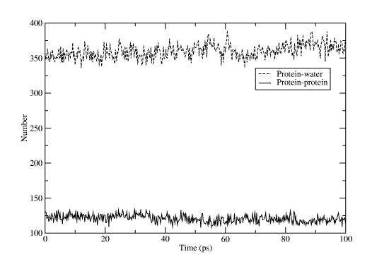
Another useful measure is the number of hydrogen bonds, both inside the protein and between protein and water atoms. Of course, there is a Gromacs program for this too:

g_hbond -s run.tpr -f run.xtc
 

Select “protein” for one group and "SOLA" for the other. Rename the output file hbnum.xvg, and then run the program again, but this time with "€œprotein" for both groups. If you open one file in Grace and then import the other one as an additional set you will get something like Figure Four. That wasn't too hard, was it? Don't forget that most Gromacs programs have a huge list of options to alter their behavior, and if the predefined groups don't match your needs you can easily create a custom index file with the program make_ndx!

Exporting the Trajectory for Pymol

Pymol is a great visualization program, but we need to massage the trajectory a bit before we can create really nice movies. First we will apply a lowpass filter to the trajectory to remove nice and make the atoms move more smoothly. As usual, Gromacs has a special program to do this:

g_filter -s run.tpr -f run.xtc -ol lowpass.xtc -nx 10 -all

This time we won't tell you what all the options do, find out yourself instead by executing g_filter -h! Pymol cannot read Gromacs xtc trajectories (yet), and we also want to remove all the water in the trajectory to concentrate on the proteins. This is easy to fix by using another Gromacs program to convert the trajectory to PDB format and only select one group:

trjconv -s run.tpr -f lowpass.xtc -o lzmtraj.pdb

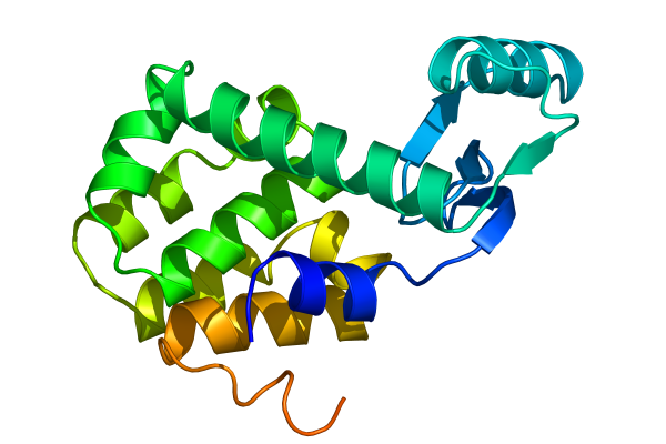
Select “protein” when asked for an output group, and visualize the resulting trajectory with the command pymol lzmtraj.pdb. You can push the VCR-style buttons in Pymol to play back the trajectory, and if you really want to impress the audience at a talk you should choose to raytrace/render all frames from the movie menu. If you are using a Macintosh, Pymol can save the movie directly in quicktime format. Otherwise you will need to export a series of images and use an external program to create a movie. Figure Five shows the last frame of a movie we made of the tutorial simulation!

Other Programs

Gromacs is a pretty big package with more than 70 analysis programs, so we've really only scratched the surface here. Make sure you check out the options to the existing programs before you start writing your own code from the included template source. Some of the tools we find most useful are:

• g_gyrate to calculate radii of gyration, both average and around the x/y/z axes.
• g_bond and g_angle to calculate values and averages of arbitrary distances and angles over time in a trajectory.
• trjorder to reorder the atoms in an arbitrary group in a trajectory with respect to the distance to another arbitrary group. This way you can create a trajectory with only a first hydration shell of water, or the water close to an active site.
• g_rama to calculate values of phi/psi backbone dihedrals as a function of time.
• g_cluster to cluster structures in a trajectory with several different algorithms, and to calculate the distances between these clusters.
• do_dssp is a wrapper around the dssp program to create secondary structure plots as a function of time for proteins.
• g_msd calculates mean square displacements and does automatic fitting to calculate diffusion coefficients for different groups.
• g_sas to compute hydrophobic, hydrophilic and total solvent accessible surface area.
• g_order if you need to determine order parameters, in particular for lipid bilayers.
• g_velacc for autocorrelation functions of atoms or molecules, both velocity and momentum.

Improving Parallel Performance

We all want better performance, don't we? Since parallel molecular dynamics involves large amounts of communication between nodes for each step, the underlying hardware and MPI library will have a very direct effect on communication and thus on your total simulation performance. Small systems (less than 10,000 atoms) are usually most sensitive to the latency, while larger simulations (100,000 atoms or more) also need high bandwidth to send all the data each step. This section is a summary of some of the things we've learned from our own cluster experience, many of them are not specific to Gromacs, but should apply to parallel programs in general. You can safely skip it if you are a novice, but read on if you are building a new cluster or would like your current network to perform better.

Hardware Considerations

Gromacs comes with manually tuned assembly loops for a wide range of hardware. AMD Opteron CPUs currently provide the best price/performance ratio, closely followed by IBM PowerPC 970 (Apple G5) and Intel Xeon/Pentium IV. If you are building your own cluster for the first time it might still be a good idea to use Xeon, simply because it is the oldest and most tested architecture. We strongly recommend that you use SMP (dual) machines in the cluster since the shared-memory communication between the CPUs has extremely low latency and high bandwidth -- and they are cheaper than two single-CPU boxes.

For SMP Xeons, it is important to turn OFF hyperthreading in the bios. This might seem like incredibly stupid advice, since four processors should be better than two, right? Unfortunately, the Linux kernel (including version 2.6) still has problems to do proper scheduling with hyperthreading: If you run two jobs, they sometimes end up on the two virtual CPUs sharing inside one physical CPU, while the other physical CPU is idle. You can imagine what this does to your performance, so just say no to hyperthreading for now. Even if the Linux scheduler did a perfect job you would not see much difference for CPU-bound programs like Gromacs - the integer and floating-point units are not duplicated in current Xeon implementations.

It is a good idea to have some sort of network between the nodes in your cluster. If you have a deep wallet or can apply for time at existing supercomputer facilities, the best solution is to use a dedicated high-performance interconnect such as Myrinet, Infiniband or Scali that provide both low latency and high bandwidth. All these vendors provide their own MPI libraries and documentation, so in that case you should stop reading this and instead ask the vendor how to get the best possible performance. If you are spending your own funds the situation is a little more complex. Myrinet or the alternatives might still be worth it in some cases, but due to the fairly high price we often accept standard Gigabit Ethernet so we can buy more nodes instead.

Tweaking Your MPI Library

What if you already have a cheap Ethernet-based cluster that you would like to be faster, but you're not willing to spend a single cent? Fortunately there are some free lunches in the Free Software world! MPI over Ethernet is slow because it usually involves copying data to a temporary buffer and then calling the Linux network card drivers, and vice versa at the receiving node. If the message is larger than the "€œsmall message" buffer size we must first send a header message warning that a large message will follow. This is portable and resource-efficient, but you can probably imagine what it does to your performance. Let's see what can be done about it. First, if you are running Linux there are special MPI implementations (MPI/GAMMA or Scali MPI Connect) that can talk directly to a small number of network cards and bypass the driver. Check them out with Google and compare to your hardware. If your system is supported you could achieve latencies as low as 10 microseconds!

Unfortunately the special libraries do not support the gigabit cards in our nodes, so we have to stick with LAM/MPI, which we have found to be a tiny bit faster than MPICH. You may want to explore the next generation MPI's such as MPICH2 and Open MPI as well. However, even in the case of LAM/MPI it is well worth recompiling the library with better options. By default TCP/IP communication is used between all processes, but you most certainly want to use shared memory instead when two processes are on the same node. You should also increase the “small message” buffer size significantly. Download the source from the LAM site and configure it as

./configure -prefix=/home/joe/software \
            -with-rpi=usysv            \
            -with-tcp-short=524288     \
            -with-shm-short=524288

Here we assumed you do not have root privileges, but want to install the software under your home directory /home/joe. Issue make and then make install, and your new tweaked MPI library is ready to use once you add /home/joe/software/bin to your path.

Your Batch Queue System

Ideally the batch system should optimize the allocation if you for instance ask for 8 processors, but in practice it is more or less random. You want to make sure the 8 processors are confined 4 SMP nodes where you have both CPUs, and in a large cluster with one switch per rack all the nodes should be in the same rack so you only have a single switch between them. For the PBS and Torque queue systems this can be accomplished with a batch submission command like

qsub -l nodes=4:rack1:ppn=2 script

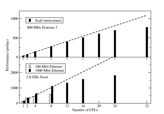
This command only works if the property “rack1” is assigned to all nodes in rack1. If it's not done on your cluster, bug the administrator until it is fixed -- this is a big performance gain compared to running on single processors per node spread over two or more racks. Figure Six shows some results for the standard Gromacs scaling benchmark -- a 130,000-atom DPPC membrane system with long electrostatics cut-offs.

Conclusions

The simulation process described here is quite typical: an initial energy minimization followed by equilibration with position restraints, although the equilibration could be a bit longer in practice. Since the first part of the non-restrained simulation should also be discarded as equilibration in practice, it is common to perform another free simulation with pressure coupling (to achieve the right density) before the production run starts, but we simply didn't have room for that in this tutorial!

When you start your own simulations, remember to be gentle with your proteins and don't neglect warning messages -- there is a reason why they are there. Unfortunately simulations are actually very much like laboratory experiments: it is very easy to destroy months of work with a moment of recklessness. There is a wealth of information available at the Gromacs website, including a paper manual and more important: several very active user mailing list. We're looking forward to see your posts there!

This article was originally published in ClusterWorld Magazine. It has been updated and formatted for the web. If you want to read more about HPC clusters and Linux you may wish to visit Linux Magazine.

Erik Lindahl is a Gromacs co-author and assistant professor at the Stockholm Bioinformatics Institute, Sweden.