The Production Simulation
After the position restrained equilibration has finished it is time for the real simulation where we will collect data to analyze. We will disable position restraints, generate more output data, and use the velocities from the end of the last simulation (saved in the .gro file) instead of generating new ones. The contents of run.mdp is:integrator = md nsteps = 50000 dt = 0.002 nstxout = 10000 nstvout = 10000 nstxtcout = 100 nstlog = 1000 nstenergy = 100 energygrps = protein sol rlist = 1.0 coulombtype = cut-off rcoulomb = 1.0 vdwtype = cut-off rvdw = 1.0 tcoupl = berendsen tc-grps = system tau-t = 0.1 ref-t = 298 constraints = h-bonds
The total simulation time is 100 ps (50,000 steps), which is still very short but enough for a tutorial. Every 10,000 steps we save full precision coordinates and velocities to the trajectory run.trr so we can restart the simulation if something goes wrong, and every 100 steps we will write compressed coordinates to run.xtc (10 times smaller than general trajectories). Energies and similar data like pressure is written every 100 steps to run.edr, and energy terms are written separately for all combinations between protein and solvent groups. Generate the run input file:
grompp -f run.mdp -p topol.top -c pr.gro -o run.tpr -np 4
This simulation will take a while, so let's create a script so it can be submitted as a batch job. The PBS/Torque options can be embedded as a comment in the script, and since most clusters have SMP nodes we ask for 2 nodes and 2 processors per node:
#PBS -l nodes=2:ppn=2
lamboot -v $PBS_NODEFILE
cd /your/project/directory
mpirun -np 4 /path/to/mdrun -deffnm run
wipe
Make the scriptfile executable, and submit the job as qsub scriptfile. Go and have a cup of coffee while you swear over other users competing for resources, and when you are back the output files should be ready in your project directory. All Gromacs binary files are portable, so if you want to you can copy the results and do all post-run analysis on your workstation if Gromacs is installed there.
Analyzing The Energy File
The Gromacs energy files are a bit special in that they store partial sums of energy terms. If you used nstenergy=100 the instantaneous values are written every 100 steps, but the averages and drift statistics we extract from the file are still exact and based on every single step in the simulation. This even works if you are analyzing parts of a simulation, for instance the interval 5.0-10.0 ps in our production run. Use the Gromacs program g_energy to extract data from energy files:g_energy -f run.edr
You will be presented with a table of different energy terms, pressures, temperature, etc. Select a couple of terms you are interested in and finish with 0. g_energy will write the average, fluctuation and systematic drift to the screen, and generate the plotfile energy.xvg. Remember that we talked about the Grace program before? If you installed it you can simply type
xmgrace -nxy energy.xvg
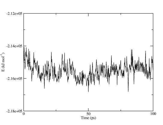
and you will get a finished graph with captions and legends. Figure Two shows the total potential energy, all we did in Grace was to make the graph a little wider. You can even use the command line options to xmgrace and produce postscript or PDF plots automatically!

Analyzing Trajectories
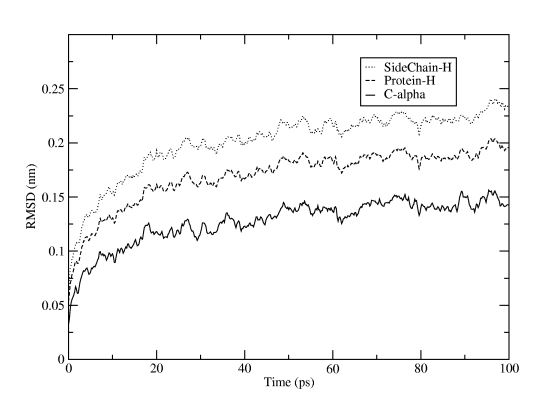
What else can we do? Well, a common property to be interested in is the RMSD variation of atoms with respect to the initial structure. Let's generate it from the trajectory:g_rms -s em.tpr -f run.xtc
The reference structure is taken from the tpr file, so we use the energy minimization run input file that started from the PDB structure. You will first be asked which group should be used for the fitting (select C-alpha), then how many groups you want to calculate RMSD for, and which these groups should be. The result will be written to rmsd.xvg, and just as for the energy file plot you can directly fire it up in xmgrace. For Figure Three we selected the three groups C-alpha, the whole protein (except for hydrogens), and only sidechains (except for hydrogens).

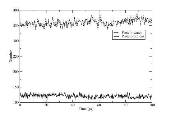
Another useful measure is the number of hydrogen bonds, both inside the protein and between protein and water atoms. Of course, there is a Gromacs program for this too:
g_hbond -s run.tpr -f run.xtc
Select âproteinâ for one group and "SOLA" for the other. Rename the output file hbnum.xvg, and then run the program again, but this time with "protein" for both groups. If you open one file in Grace and then import the other one as an additional set you will get something like Figure Four. That wasn't too hard, was it? Don't forget that most Gromacs programs have a huge list of options to alter their behavior, and if the predefined groups don't match your needs you can easily create a custom index file with the program make_ndx!

Exporting the Trajectory for Pymol
Pymol is a great visualization program, but we need to massage the trajectory a bit before we can create really nice movies. First we will apply a lowpass filter to the trajectory to remove nice and make the atoms move more smoothly. As usual, Gromacs has a special program to do this:g_filter -s run.tpr -f run.xtc -ol lowpass.xtc -nx 10 -all
This time we won't tell you what all the options do, find out yourself instead by executing g_filter -h! Pymol cannot read Gromacs xtc trajectories (yet), and we also want to remove all the water in the trajectory to concentrate on the proteins. This is easy to fix by using another Gromacs program to convert the trajectory to PDB format and only select one group:
trjconv -s run.tpr -f lowpass.xtc -o lzmtraj.pdb
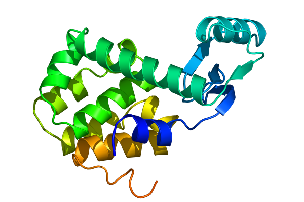
Select âproteinâ when asked for an output group, and visualize the resulting trajectory with the command pymol lzmtraj.pdb. You can push the VCR-style buttons in Pymol to play back the trajectory, and if you really want to impress the audience at a talk you should choose to raytrace/render all frames from the movie menu. If you are using a Macintosh, Pymol can save the movie directly in quicktime format. Otherwise you will need to export a series of images and use an external program to create a movie. Figure Five shows the last frame of a movie we made of the tutorial simulation!

Other Programs
Gromacs is a pretty big package with more than 70 analysis programs, so we've really only scratched the surface here. Make sure you check out the options to the existing programs before you start writing your own code from the included template source. Some of the tools we find most useful are:- g_gyrate to calculate radii of gyration, both average and around the x/y/z axes.
- g_bond and g_angle to calculate values and averages of arbitrary distances and angles over time in a trajectory.
- trjorder to reorder the atoms in an arbitrary group in a trajectory with respect to the distance to another arbitrary group. This way you can create a trajectory with only a first hydration shell of water, or the water close to an active site.
- g_rama to calculate values of phi/psi backbone dihedrals as a function of time.
- g_cluster to cluster structures in a trajectory with several different algorithms, and to calculate the distances between these clusters.
- do_dssp is a wrapper around the dssp program to create secondary structure plots as a function of time for proteins.
- g_msd calculates mean square displacements and does automatic fitting to calculate diffusion coefficients for different groups.
- g_sas to compute hydrophobic, hydrophilic and total solvent accessible surface area.
- g_order if you need to determine order parameters, in particular for lipid bilayers.
- g_velacc for autocorrelation functions of atoms or molecules, both velocity and momentum.


